


Estimating Models with Significant Initial Conditions
Thursday, 18 October 2012
Normally, when using rivbj and rivcbj routines in CAPTAIN, it is assumed that the data will be selected or edited so that the initial conditions are near zero. However, in situations where these initial conditions are important in themselves, it is possible to estimate them buy using the multiple input option. Of course, this has been available as an option for a long time in these routines but it has come to my attention that it is not well known.

For example, consider a simulation model that relates to a model of effective rainfall u(t) to flow x(t) in a river, with a pronounced initial flow condition so that the estimation results are much better if this IC is taken into account. The transfer function model is as follows:

where s=d/dt is the differential operator. White noise is added to the simulated flow x(t) to yield a measured output y(t) with a 20% noise level by standard deviation. The motivation for the approach is the Laplace transform of the differential equation associated with the above transfer function. This has the same form as the above transfer function equation but with additional additive terms arising from any initial conditions on the variables and their derivatives. It is these initial condition terms that are handled by the additional input. I will leave the reader to think about this, based on the results below.
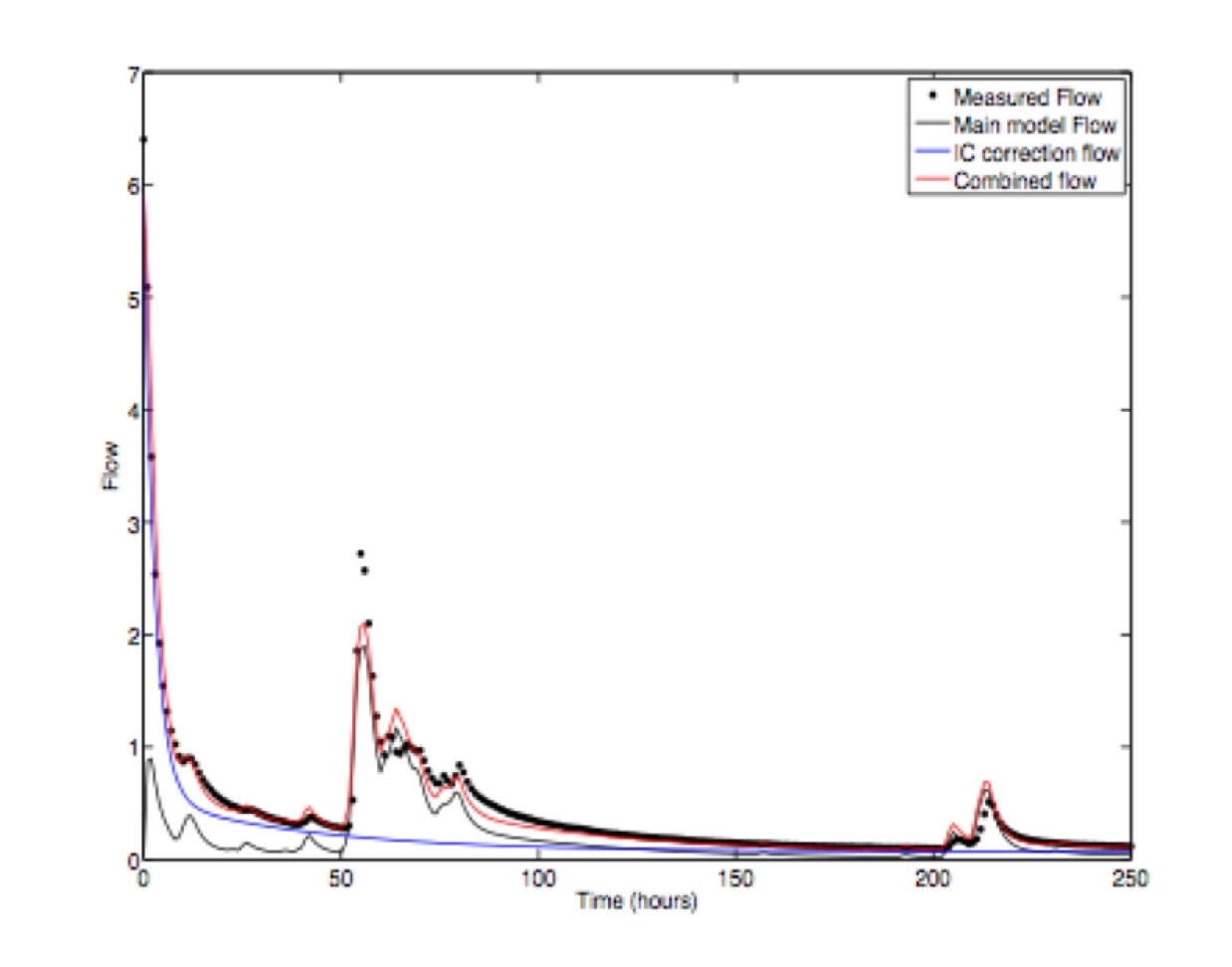
The first figure shows the results of estimating this model with two inputs using the following call to the rivcbj routine in CAPTAIN:
[thc,Mc,Mnc,Dc,statsc,ec,eefc,varc,Psc,Pnc] =...
rivcbj([yh ues ones(size(yh))],[2 3 3 0 0 0 0],[0.00001 1 1 0],-0.1)
Here, the second input is simply a vector of ones of the same size as x(t). The ‘main model flow’ response to the first input u(t) starts with zero initial conditions. However, the ‘IC correction flow’ response to the second, unity input produces a marked initial condition induced response that, when added to the main model flow, yields a combined input that explains the noisy measured data well, with a coefficient of determination of 0.96, in relation to the noisy data, and virtually 1.0 in relation to the noise-free data: i.e. the estimated model output is virtually the same as x(t).
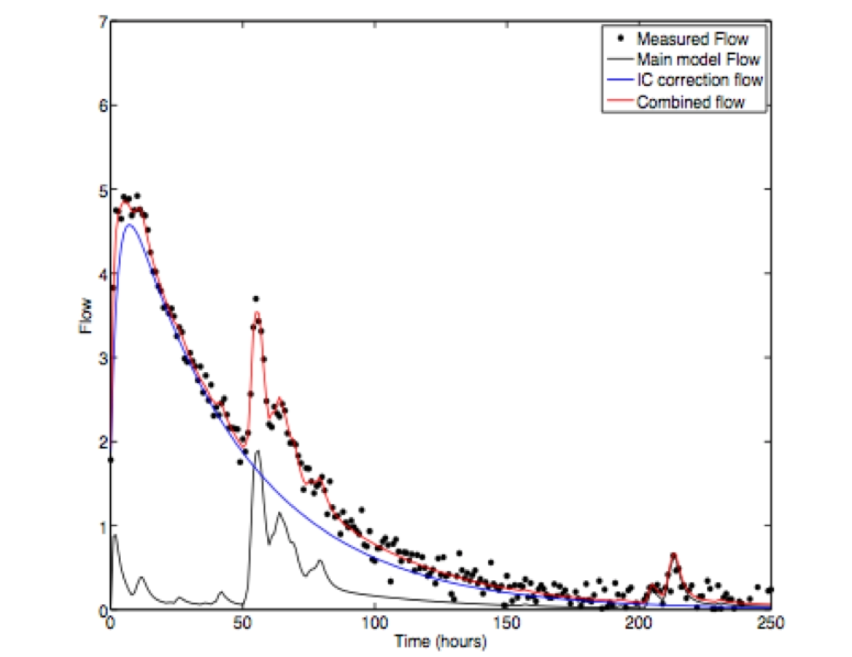
The second figure shows this same approach applied to real effective rainfall-flow data, where the initial condition does not have such a large effect but the estimation again works well.